Today, in the data-driven world, many organizations strive on the data and statistical techniques to get the insights of data. Logistic regression is one such technique used to calculate the probability of default. A very simple example could be email classification with some given set of attributes like links ,words in mail body, images etc to decide whether the emails are spam(0) or not(1).
Now, let’s understand what is logistic regression ?
Logistic regression known as the logit model, is used to model binary result variables. In the logit model, the log odds of the result is displayed as a linear combination of the independent variables. It is one of the most commonly used methods in statistics to predict a real-valued result. Logistic regression is an analytical method to examine/predict the direct relationship within an independent variable and dependent variables. This is a simple process that takes real value inputs to make a prediction on the probability of the input variable. On the contrary, the logistics regression can sometimes becomes classification techniques only when the threshold of the decision comes into the picture. The threshold value depends on classification problem itself.
Logistic regression considers the probability of the dependent variable and uses GLM() function that uses:
p: the probability of success
(1-p): the probability of failure
Where p should be positive (p >= 0) and should be less than 1 (p <= 1)
GLM ( ) function is known as generalized linear model which is generalization of simple linear function helps in analysing the linear relationship between the response variable and the continuous or categorical independent variables.Generalized Linear Models are an expansion of the linear model framework, which incorporates dependent variables which are not normally distributed. They hold three features:
-
The models include a linear combination of independent variables.
-
The mean of the binary dependent variable is linked to the linear combination of independent variables.
3. The dependent variable is said to follow binary distribution which belongs to the family of exponential distribution.
Assumptions of Logistic Regression
Logistic regression is a particular case of the generalized linear model where the dependent variable or response variable is either a 0 or 1. It returns the target variables as probability values. But we can transform and obtain the benefits using threshold value. To apply logistic regression few assumptions were made:-
-
The dependent or response variable should be binomially distributed.
-
There should be a linear relationship between the independent variables and the logit or link function.
-
The response variable should be mutually exclusive.
Now you might wonder what it Binomial distributions as the response variable is binomially distributed. Let’s get basic idea of binomial distribution :-
-
The binomial distribution contains a fixed number of trails.
-
Each trial has only two possible outcomes, i.e. failure or success.
-
The probability of the outcome of any trail (toss) remains fixed over time.
-
The trials are statistically independent .i.e the outcomes of one toss does not affect the outcome of any other toss.
What are the advantages of using logistic regression ?
Logistic regression is the most powerful technique used in credit lending business which helps in developing scorecard to measure the probability of default. The binary response variable helps to depict the probability of defaulting in future thereby reducing the risk.
The main advantage of logistic regression is that we can include more than one dependent variable which could be ordinal or dichotomous (binary) make it more apt to use over chi square test. Another advantage of using logistic regression is that it quantifies the strength of association with other variables.
Here comes the interesting part ! How logistic regression work?
The logit function used in the computation is :-
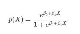
The above equation can be transformed :
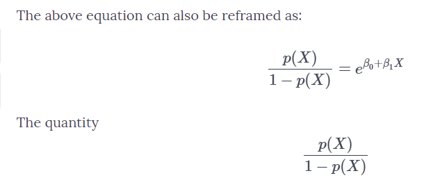
The logit function ranges from −∞ to ∞ and takes a value between 0 to 1.
Taking log on both sides the final equation can be written as :-

Now , taking the inverse to calculate the P(X) = exp(βˆtx)
1+ exp(βˆ tx)
Pitfalls and Caution while implementing Logistic Regression
-
Selection of variables:
While performing any research is important to consider all the aspects by taking as many variables as possible, but this could lead to large standard errors and also affect the true relation or identify meretricious associations. So to prevent this its advisable to use univariate analysis with each input variable and check the significance cutoff and then thereby including or rejecting particular variable the cutoff value should p<0.10 rather than p<0.05 traditionally. This will help the researcher to separate the potential predictors from the set of all the input variables to include in logistic regression. Therefore it's advisable to choose the right input variables for accurate results.
-
Rejecting highly correlated variables:
It's important or any researcher to check the correlation between the input variables generally known as as it affects the model making it less precise. For instance, let's take age, height and body surface area as input variables to measure the rate of developing hypertension. As height and body surface area have a high correlation with one another. In such a scenario, the regression model should consider only one of the two interrelated input variables for more processed outputs.
-
Handle continuous predictor or independent variables.
In case the input variables are continuous for example weight or height then we can either convert them into a categorical variable like height>5 or height <=5. Though it's not a good practice as some part of the information is lost while converting.
Implementation in R
Let's apply logistic regression in R by considering an example to measure the rate of defaulting a bank loan using age, area, education,cibil_score, equifax_score,no_of_dependents, profession as input variables. Perform logistic regression to check whether the person will default in future(1) or not(0).
Set the working directory where all the outputs and scripts will be saved for future reference and then download and load the libraries to perform the logistic regression
> path <- "apurva/Data/new"
> setwd(location or path)
> library (plyr)
> library (data.table)
> library (stringr)--- # load the library
Load the files with names train1 and test1 in csv format using fread function. And then to see the values use head function() and summary () function
> train1 <- read.csv("train1.csv",na.strings = c(""," ",NA,"NA"))
> test1 <- read.csv("test1.csv",na.strings = c(""," ",NA,"NA"))
> print(train1)
> print(test1)
> head(train1)
> head(test1)
> str(test1)
> str(train1)
Use data manipulation techniques to check the missing values and treating outliers :
This step is the most important part of any analysis as it is extremely important to check the descriptive statistics , missing values
> colsums(is.na(train1))
> colsums(is.na(test1))
> summary(train1$A)
Combine the data as per your requirement and then combine the tiles as per needed
> newdata <- rbind(train1,test1,fill=TRUE)
> newdata [,title: =replace(title1, which(title1 %in%c("age","area","education","cibil_score","profession","no_of_dependents",”equifax_score”)),"rs"),by=title]
Training and Test Samples:Now, in order to perform logistic regression the sample is divided into two trains and test sample:
> train1 <-newdata[!(is.na(NEW))]
> train1 [,NEW := as.factor(NEW)]
> test1 <- newdata[is.na(NEW)]
> test1 [,NEW := NULL]
Now, using the glm () function to run the model and use summary() function
#logistic regression model
##>modellog<-glm(Recommended~age+area+education+cibil_score+equifa##>x_score+no_of_dependents+profession, data = train1,family = ##>binomial)
##>summary(modellog)
# Deviance Residuals:
## Min 1Q Median 3Q Max
## -1.527 -0.476 -0.636 1.149 2.079
##
## Coefficients:
## Estimate Std. Error z value Pr(>|z|)
## (Intercept) -3.98998 1.13995 -3.50 0.00047 ***
## age 0.0665 0.00109 2.07 0.03847 *
## area 0.80404 0.33182 2.42 0.01689 *
## cibil_score -0.67544 0.31649 -2.13 0.03283 **
## education -1.31520 0.34531 -3.88 0.00020 *
## profession -1.55146 0.41783 -3.71 0.00010 **
## no_of_dependents -1.11520 0.53125 -5.28 0.001000 **
## equifax_score 0.8504 0.53182 3.42 0.01689 ***
## ---
## Signif. codes: 0 '*' 0.001 '*' 0.01 '***' 0.05 '.' 0.1 ' ' 1
##
## (Dispersion parameter for binomial family taken to be 1)
##
## Null deviance:489.32 on 398 degrees of freedom
## Residual deviance:428.26 on 365 degrees of freedom
## AIC: 470.5
AIC value of the model is 470.5 and we the estimates of all the independent variable and so now we can calculate the probability of each response. AIC is measured the same way as R squared in multiple regression model. The thumb rule to AIC is that the smaller value has a high accuracy better it is.
log p /1 − p = 1.8185 − 0.0665 × Age
Probability of default :
log p /(1 − p) = 1.81 − 0.06455 × 0
p/ (1 − p) = exp(1.81) = 6.26 p = 6.26/7.56 = 0.81
Check the accuracy of the model?
To check the predictability and reliability of the model use ROC Curve
Note: ROC is an area under the curve which gives us the accuracy of the model. Its is also known as the index of accuracy which represents the performance.
More the area under the curve, the better the model. Graphically it is represented using two-axis one is true positive rate and false positive Y and X-axis respectively. The value should approaches 1 in order to have a better model.
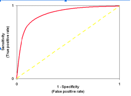
Download and use the download ROCR library
plot ROC -- load library
> library (Metrics)
> library(ROCR)
> pr <- prediction ( log$predict,test$NEW)
> performance1 < - performance(y,measure = "tr",tr.measure = "fr")
> plot(performance1) > auc(test$1new,log_predict)
ROC is 0.76 implies that the model is predicting negative values incorrectly. GLM () model does not assume that there is any linear relationship between independent or dependent variables. Nevertheless, it does assume a linear relationship between link function and independent variables in the logistic model.
The blog is intended to help people learn and perform Logistic Regression in R. Understanding Logistic Regression has its own difficulties. It is quite similar to Multiple Regression but differs in the way a response variable is predicted or evaluated.
While working on a classification problem. I would recommend you to develop your first model as Logistic Regression. The reason being that you might score a remarkable efficiency even better than non-linear methods. While reading and practising this tutorial, if there is anything you don't know, don't wait to drop in your comments below!